1.介绍
有三种不同的方法来评估一个模型的预测质量:
- estimator的score方法:sklearn中的estimator都具有一个score方法,它提供了一个缺省的评估法则来解决问题。
- Scoring参数:使用cross-validation的模型评估工具,依赖于内部的scoring策略。见下。
- Metric函数:metrics模块实现了一些函数,用来评估预测误差。见下。
2. scoring参数
模型选择和评估工具,例如: grid_search.GridSearchCV 和 cross_validation.cross_val_score,使用scoring参数来控制你的estimator的好坏。
2.1 预定义的值
对于大多数case而说,你可以设计一个使用scoring参数的scorer对象;下面展示了所有可能的值。所有的scorer对象都遵循:高得分,更好效果。如果从mean_absolute_error 和mean_squared_error(它计算了模型与数据间的距离)返回的得分将被忽略。

2.2 从metric函数定义你的scoring策略
sklearn.metric提供了一些函数,用来计算真实值与预测值之间的预测误差:
- 以_score结尾的函数,返回一个最大值,越高越好
- 以_error结尾的函数,返回一个最小值,越小越好;如果使用make_scorer来创建scorer时,将greater_is_better设为False
接下去会讨论多种机器学习当中的metrics。
许多metrics并没有给出在scoring参数中可配置的字符名,因为有时你可能需要额外的参数,比如:fbeta_score。这种情况下,你需要生成一个合适的scorer对象。最简单的方法是调用make_scorer来生成scoring对象。该函数将metrics转换成在模型评估中可调用的对象。
第一个典型的用例是,将一个库中已经存在的metrics函数进行包装,使用定制参数,比如对fbeta_score函数中的beta参数进行设置:
>>> from sklearn.metrics import fbeta_score, make_scorer
>>> ftwo_scorer = make_scorer(fbeta_score, beta=2)
>>> from sklearn.grid_search import GridSearchCV
>>> from sklearn.svm import LinearSVC
>>> grid = GridSearchCV(LinearSVC(), param_grid={'C': [1, 10]}, scoring=ftwo_scorer)
第二个典型用例是,通过make_scorer构建一个完整的定制scorer函数,该函数可以带有多个参数:
- 你可以使用python函数:下例中的my_custom_loss_func
- python函数是否返回一个score(greater_is_better=True),还是返回一个loss(greater_is_better=False)。如果为loss,python函数的输出将被scorer对象忽略,根据交叉验证的原则,得分越高模型越好。
- 对于分类问题的metrics:如果你提供的python函数是否需要对连续值进行决策判断,可以将参数设置为(needs_threshold=True)。缺省值为False。
- 一些额外的参数:比如f1_score中的bata或labels。
下例使用定制的scorer,使用了greater_is_better参数:
>>> import numpy as np
>>> def my_custom_loss_func(ground_truth, predictions):
...     diff = np.abs(ground_truth - predictions).max()
...     return np.log(1 + diff)
...

>>> loss  = make_scorer(my_custom_loss_func, greater_is_better=False)
>>> score = make_scorer(my_custom_loss_func, greater_is_better=True)
>>> ground_truth = [[1, 1]]
>>> predictions  = [0, 1]
>>> from sklearn.dummy import DummyClassifier
>>> clf = DummyClassifier(strategy='most_frequent', random_state=0)
>>> clf = clf.fit(ground_truth, predictions)
>>> loss(clf,ground_truth, predictions)
-0.69...
>>> score(clf,ground_truth, predictions)
0.69...
2.3 实现你自己的scoring对象
你可以生成更灵活的模型scorer,通过从头构建自己的scoring对象来完成,不需要使用make_scorer工厂函数。对于一个自己实现的scorer来说,它需要遵循两个原则:
- 必须可以用(estimator, X, y)进行调用
- 必须返回一个float的值
3. 分类metrics
sklearn.metrics模块实现了一些loss, score以及一些工具函数来计算分类性能。一些metrics可能需要正例、置信度、或二分决策值的的概率估计。大多数实现允许每个sample提供一个对整体score来说带权重的分布,通过sample_weight参数完成。
一些二分类(binary classification)使用的case:
- matthews_corrcoef(y_true, y_pred)
- precision_recall_curve(y_true, probas_pred)
- roc_curve(y_true, y_score[, pos_label, …])
一些多分类(multiclass)使用的case:
- confusion_matrix(y_true, y_pred[, labels])
- hinge_loss(y_true, pred_decision[, labels, …])
一些多标签(multilabel)的case:
- accuracy_score(y_true, y_pred[, normalize, …])
- classification_report(y_true, y_pred[, …])
- f1_score(y_true, y_pred[, labels, …])
- fbeta_score(y_true, y_pred, beta[, labels, …])
- hamming_loss(y_true, y_pred[, classes])
- jaccard_similarity_score(y_true, y_pred[, …])
- log_loss(y_true, y_pred[, eps, normalize, …])
- precision_recall_fscore_support(y_true, y_pred)
- precision_score(y_true, y_pred[, labels, …])
- recall_score(y_true, y_pred[, labels, …])
- zero_one_loss(y_true, y_pred[, normalize, …])
还有一些可以同时用于二标签和多标签(不是多分类)问题:
- average_precision_score(y_true, y_score[, …])
- roc_auc_score(y_true, y_score[, average, …])
在以下的部分,我们将讨论各个函数。
3.1 二分类/多分类/多标签
对于二分类来说,必须定义一些matrics(f1_score,roc_auc_score)。在这些case中,缺省只评估正例的label,缺省的正例label被标为1(可以通过配置pos_label参数来完成)
将一个二分类matrics拓展到多分类或多标签问题时,我们可以将数据看成多个二分类问题的集合,每个类都是一个二分类。接着,我们可以通过跨多个分类计算每个二分类metrics得分的均值,这在一些情况下很有用。你可以使用average参数来指定。
- macro:计算二分类metrics的均值,为每个类给出相同权重的分值。当小类很重要时会出问题,因为该macro-averging方法是对性能的平均。另一方面,该方法假设所有分类都是一样重要的,因此macro-averaging方法会对小类的性能影响很大。
- weighted: 对于不均衡数量的类来说,计算二分类metrics的平均,通过在每个类的score上进行加权实现。
- micro: 给出了每个样本类以及它对整个metrics的贡献的pair(sample-weight),而非对整个类的metrics求和,它会每个类的metrics上的权重及因子进行求和,来计算整个份额。Micro-averaging方法在多标签(multilabel)问题中设置,包含多分类,此时,大类将被忽略。
- samples:应用在 multilabel问题上。它不会计算每个类,相反,它会在评估数据中,通过计算真实类和预测类的差异的metrics,来求平均(sample_weight-weighted)
- average:average=None将返回一个数组,它包含了每个类的得分.
多分类(multiclass)数据提供了metric,和二分类类似,是一个label的数组,而多标签(multilabel)数据则返回一个索引矩阵,当样本i具有label j时,元素[i,j]的值为1,否则为0.
3.2 accuracy_score
accuracy_score函数计算了准确率,不管是正确预测的fraction(default),还是count(normalize=False)。
在multilabel分类中,该函数会返回子集的准确率。如果对于一个样本来说,必须严格匹配真实数据集中的label,整个集合的预测标签返回1.0;否则返回0.0.
预测值与真实值的准确率,在n个样本下的计算公式如下:
\[accuracy(y,\hat{y}) = \frac{1}{n_{samples}} \sum_{i=0}^{n_{samples}-1}l(\hat{y}_i=y_i)\]1(x)为指示函数。
>>> import numpy as np
>>> from sklearn.metrics import accuracy_score
>>> y_pred = [0, 2, 1, 3]
>>> y_true = [0, 1, 2, 3]
>>> accuracy_score(y_true, y_pred)
0.5
>>> accuracy_score(y_true, y_pred, normalize=False)
2
在多标签的case下,二分类label:
>>> accuracy_score(np.array([[0, 1], [1, 1]]), np.ones((2, 2)))
0.5
3.3 Cohen’s kappa
函数cohen_kappa_score计算了Cohen’s kappa估计。这意味着需要比较通过不同的人工标注(numan annotators)的标签,而非分类器中正确的类。
kappa score是一个介于(-1, 1)之间的数. score>0.8意味着好的分类;0或更低意味着不好(实际是随机标签)
Kappa score可以用在二分类或多分类问题上,但不适用于多标签问题,以及超过两种标注的问题。
3.4 混淆矩阵
confusion_matrix函数通过计算混淆矩阵,用来计算分类准确率。
缺省的,在混淆矩阵中的i,j指的是观察的数目i,预测为j,示例:
>>> from sklearn.metrics import confusion_matrix
>>> y_true = [2, 0, 2, 2, 0, 1]
>>> y_pred = [0, 0, 2, 2, 0, 2]
>>> confusion_matrix(y_true, y_pred)
array([[2, 0, 0],
       [0, 0, 1],
       [1, 0, 2]])
结果为:

示例:
- Confusion matrix
- Recognizing hand-written digits
- Classification of text documents using sparse features
3.5 分类报告
classification_report函数构建了一个文本报告,用于展示主要的分类metrics。 下例给出了一个小示例,它使用定制的target_names和对应的label:
>>> from sklearn.metrics import classification_report
>>> y_true = [0, 1, 2, 2, 0]
>>> y_pred = [0, 0, 2, 2, 0]
>>> target_names = ['class 0', 'class 1', 'class 2']
>>> print(classification_report(y_true, y_pred, target_names=target_names))
             precision    recall  f1-score   support

    class 0       0.67      1.00      0.80         2
    class 1       0.00      0.00      0.00         1
    class 2       1.00      1.00      1.00         2

avg / total       0.67      0.80      0.72         5
示例:
3.6 Hamming loss
hamming_loss计算了在两个样本集里的平均汉明距离或平均Hamming loss。
- $ \hat{y}_j $是对应第j个label的预测值,
- $ y_j $是对应的真实值
- $ n_\text{labels} $是类目数
那么两个样本间的Hamming loss为$ L_{Hamming} $,定义如下:
\[L_{Hamming}(y, \hat{y}) = \frac{1}{n_\text{labels}} \sum_{j=0}^{n_\text{labels} - 1} 1(\hat{y}_j \not= y_j)\]其中:$ 1(x) $为指示函数。
>>> from sklearn.metrics import hamming_loss
>>> y_pred = [1, 2, 3, 4]
>>> y_true = [2, 2, 3, 4]
>>> hamming_loss(y_true, y_pred)
0.25
在多标签(multilabel)的使用二元label指示器的情况:
>>> hamming_loss(np.array([[0, 1], [1, 1]]), np.zeros((2, 2)))
0.75
注意:在多分类问题上,Hamming loss与y_true 和 y_pred 间的Hamming距离相关,它与0-1 loss相类似。然而,0-1 loss会对不严格与真实数据集相匹配的预测集进行惩罚。因而,Hamming loss,作为0-1 loss的上界,也在0和1之间;预测一个合适的真实label的子集或超集将会给出一个介于0和1之间的Hamming loss.
3.7 Jaccard相似度系数score
jaccard_similarity_score函数会计算两对label集之间的Jaccard相似度系数的平均(缺省)或求和。它也被称为Jaccard index.
第i个样本的Jaccard相似度系数(Jaccard similarity coefficient),真实标签集为$ y_i $,预测标签集为:$ \hat{y}_j $,其定义如下:
\[J(y_i, \hat{y}_i) = \frac{|y_i \cap \hat{y}_i|}{|y_i \cup \hat{y}_i|}.\]在二分类和多分类问题上,Jaccard相似度系数score与分类的正确率(accuracy)相同:
>>> import numpy as np
>>> from sklearn.metrics import jaccard_similarity_score
>>> y_pred = [0, 2, 1, 3]
>>> y_true = [0, 1, 2, 3]
>>> jaccard_similarity_score(y_true, y_pred)
0.5
>>> jaccard_similarity_score(y_true, y_pred, normalize=False)
2
在多标签(multilabel)问题上,使用二元标签指示器:
>>> jaccard_similarity_score(np.array([[0, 1], [1, 1]]), np.ones((2, 2)))
0.75
3.8 准确率,召回率与F值
准确率(precision)可以衡量一个样本为负的标签被判成正,召回率(recall)用于衡量所有正例。
F-meature(包括:$F_\beta$和$F_1”$),可以认为是precision和recall的加权调和平均(weighted harmonic mean)。一个$ F_\beta $值,最佳为1,最差时为0. 如果$ \beta=1$,那么$ F_\beta $和$ F_1 $相等,precision和recall的权重相等。
precision_recall_curve会根据预测值和真实值来计算一条precision-recall典线。
average_precision_score则会预测值的平均准确率(AP: average precision)。该分值对应于precision-recall曲线下的面积。
sklearn提供了一些函数来分析precision, recall and F-measures值:
- average_precision_score:计算预测值的AP
- f1_score: 计算F1值,也被称为平衡F-score或F-meature
- fbeta_score: 计算F-beta score
- precision_recall_curve:计算不同概率阀值的precision-recall对
- precision_recall_fscore_support:为每个类计算precision, recall, F-measure 和 support
- precision_score: 计算precision
- recall_score: 计算recall
注意:precision_recall_curve只用于二分类中。而average_precision_score可用于二分类或multilabel指示器格式
示例:
- 使用sparse特性的文档分类
- 使用grid search corss-validation的参数估计
- Precision-Recall
- Sparse recovery: feature selection for sparse linear models
3.8.1 二分类
在二元分类中,术语“positive”和“negative”指的是分类器的预测类别(expectation),术语“true”和“false”则指的是预测是否正确(有时也称为:观察observation)。给出如下的定义:
| 实际类目(observation) | ||
|---|---|---|
| 预测类目(expectation) | TP(true positive)结果:Correct | FP(false postive)结果:Unexpected |
| FN(false negative)结果: Missing | TN(true negtive)结果:Correct |
在这个上下文中,我们定义了precision, recall和F-measure:
\[\text{precision} = \frac{tp}{tp + fp}\] \[\text{recall} = \frac{tp}{tp + fn}\] \[F_\beta = (1 + \beta^2) \frac{\text{precision} \times \text{recall}}{\beta^2 \text{precision} + \text{recall}}\]这里是一个二元分类的示例:
>>> from sklearn import metrics
>>> y_pred = [0, 1, 0, 0]
>>> y_true = [0, 1, 0, 1]
>>> metrics.precision_score(y_true, y_pred)
1.0
>>> metrics.recall_score(y_true, y_pred)
0.5
>>> metrics.f1_score(y_true, y_pred)
0.66...
>>> metrics.fbeta_score(y_true, y_pred, beta=0.5)
0.83...
>>> metrics.fbeta_score(y_true, y_pred, beta=1)
0.66...
>>> metrics.fbeta_score(y_true, y_pred, beta=2)
0.55...
>>> metrics.precision_recall_fscore_support(y_true, y_pred, beta=0.5)
(array([ 0.66...,  1.        ]), array([ 1. ,  0.5]), array([ 0.71...,  0.83...]), array([2, 2]...))


>>> import numpy as np
>>> from sklearn.metrics import precision_recall_curve
>>> from sklearn.metrics import average_precision_score
>>> y_true = np.array([0, 0, 1, 1])
>>> y_scores = np.array([0.1, 0.4, 0.35, 0.8])
>>> precision, recall, threshold = precision_recall_curve(y_true, y_scores)
>>> precision
array([ 0.66...,  0.5       ,  1.        ,  1.        ])
>>> recall
array([ 1. ,  0.5,  0.5,  0. ])
>>> threshold
array([ 0.35,  0.4 ,  0.8 ])
>>> average_precision_score(y_true, y_scores)
0.79...
3.8.2 多元分类和多标签分类
在多分类(Multiclass)和多标签(multilabel)分类问题上,precision, recall, 和 F-measure的概念可以独立应用到每个label上。有一些方法可以综合各标签上的结果,通过指定average_precision_score (只能用在multilabel上), f1_score, fbeta_score, precision_recall_fscore_support, precision_score 和 recall_score这些函数上的参数average可以做到。
注意:
- “micro”选项:表示在多分类中的对所有label进行micro-averaging产生一个平均precision,recall和F值
- “weighted”选项:表示会产生一个weighted-averaging的F值。
可以考虑下面的概念:
- y是(sample, label)pairs的预测集
- $ \hat{y} $是(sample, label)pairs的真实集
- L是labels的集
- S是labels的集
- $ \hat{y} $是y的子集,样本s,比如:$ y_s := \left{(s’, l) \in y | s’ = s \right} $
- $ y_l $表示label l的y子集
- 同样的,$ y_s $和$ y_l $都是$ \hat{y} $的子集
- $ P(A, B) := \frac{\left | A \cap B \right |}{\left |A \right |} $
- $ R(A, B) := \frac{\left | A \cap B \right |}{\left |B \right |} $ 在处理$ B = \emptyset $时方式更不同;该实现采用$ R(A, B):=0 $,且与P相类似。
- $ F_\beta(A, B) := \left(1 + \beta^2\right) \frac{P(A, B) \times R(A, B)}{\beta^2 P(A, B) + R(A, B)} $
metrics的定义如下:

代码:
>>> from sklearn import metrics
>>> y_true = [0, 1, 2, 0, 1, 2]
>>> y_pred = [0, 2, 1, 0, 0, 1]
>>> metrics.precision_score(y_true, y_pred, average='macro')
0.22...
>>> metrics.recall_score(y_true, y_pred, average='micro')
...
0.33...
>>> metrics.f1_score(y_true, y_pred, average='weighted')
0.26...
>>> metrics.fbeta_score(y_true, y_pred, average='macro', beta=0.5)
0.23...
>>> metrics.precision_recall_fscore_support(y_true, y_pred, beta=0.5, average=None)
...
(array([ 0.66...,  0.        ,  0.        ]), array([ 1.,  0.,  0.]), array([ 0.71...,  0.        ,  0.        ]), array([2, 2, 2]...))
对于多分类问题,对于一个“negative class”,有可能会排除一些标签:
>>> metrics.recall_score(y_true, y_pred, labels=[1, 2], average='micro')
... # excluding 0, no labels were correctly recalled
0.0
类似的,在数据集样本中没有出现的label不能用在macro-averaging中。
>>> metrics.precision_score(y_true, y_pred, labels=[0, 1, 2, 3], average='macro')
...
0.166...
3.9 Hinge loss
hinge_loss函数会使用hinge loss计算模型与数据之间的平均距离。它是一个单边的metric,只在预测错误(prediction erros)时考虑。(Hinge loss被用于最大间隔分类器上:比如SVM)
如果label使用+1和-1进行编码。y为真实值,w为由decision_function结出的预测决策。 hinge loss的定义如下:
\[L_\text{Hinge}(y, w) = \max\left\{1 - wy, 0\right\} = \left|1 - wy\right|_+\]如果超过两个label,由于Crammer & Singer所提到的问题 ,hinge_loss 会使用一个多元分类的变种。
如果$ y_w $是对于true label的预测判断(predicted decision),$ y_t $则是对于其他label的预测判断的最大值,而predicted decisions由多个predicted decision输出,那么多分类的hinge loss定义如下:
$ L_\text{Hinge}(y_w, y_t) = \max\left{1 + y_t - y_w, 0\right} $
二分类问题示例:
>>> from sklearn import svm
>>> from sklearn.metrics import hinge_loss
>>> X = [[0], [1]]
>>> y = [-1, 1]
>>> est = svm.LinearSVC(random_state=0)
>>> est.fit(X, y)
LinearSVC(C=1.0, class_weight=None, dual=True, fit_intercept=True,
     intercept_scaling=1, loss='squared_hinge', max_iter=1000,
     multi_class='ovr', penalty='l2', random_state=0, tol=0.0001,
     verbose=0)
>>> pred_decision = est.decision_function([[-2], [3], [0.5]])
>>> pred_decision
array([-2.18...,  2.36...,  0.09...])
>>> hinge_loss([-1, 1, 1], pred_decision)
0.3...
多分类问题示例:
>>> X = np.array([[0], [1], [2], [3]])
>>> Y = np.array([0, 1, 2, 3])
>>> labels = np.array([0, 1, 2, 3])
>>> est = svm.LinearSVC()
>>> est.fit(X, Y)
LinearSVC(C=1.0, class_weight=None, dual=True, fit_intercept=True,
     intercept_scaling=1, loss='squared_hinge', max_iter=1000,
     multi_class='ovr', penalty='l2', random_state=None, tol=0.0001,
     verbose=0)
>>> pred_decision = est.decision_function([[-1], [2], [3]])
>>> y_true = [0, 2, 3]
>>> hinge_loss(y_true, pred_decision, labels)
0.56...
3.10 Log loss
Log loss也被称为logistic回归loss,或者交叉熵loss(cross-entropy loss),用于概率估计。它通常用在(multinomial)的LR和神经网络上,以最大期望(EM:expectation-maximization)的变种的方式,用于评估一个分类器的概率输出,而非进行离散预测。
对于二元分类,true label为:$ y \in {0,1} $,概率估计为:$ p = \operatorname{Pr}(y = 1) $,每个样本的log loss是对分类器给定true label的负值log似然估计(negative log-likelihood):
$ L_{\log}(y, p) = -\log \operatorname{Pr}(y|p) = -(y \log (p) + (1 - y) \log (1 - p)) $
当扩展到多元分类(multiclass)上时。可以将样本的true label编码成1-of-K个二元指示器矩阵Y,如果从label K集合中取出的样本i,对应的label为k,则$ y_{i,k} = 1 $,P为概率估计矩阵,$ p_{i,k} = \operatorname{Pr}(t_{i,k} = 1) $。整个集合的log loss表示如下:
\[L_{\log}(Y, P) = -\log \operatorname{Pr}(Y|P) = - \frac{1}{N} \sum_{i=0}^{N-1} \sum_{k=0}^{K-1} y_{i,k} \log p_{i,k}\]我们再看下如何对二分类的log loss进行泛化的,注意,在二分类问题上,$ p_{i,0} = 1 - p_{i,1} $ 和$ y_{i,0} = 1 - y_{i,1} $,因而,通过在$ y_{i,k} \in {0,1} $扩展内部和来给出二分类的log loss。
log_loss函数,通过给定一列真实值label和一个概率矩阵来计算log loss,返回值通过estimator的predict_proba返回。
>>> from sklearn.metrics import log_loss
>>> y_true = [0, 0, 1, 1]
>>> y_pred = [[.9, .1], [.8, .2], [.3, .7], [.01, .99]]
>>> log_loss(y_true, y_pred)
0.1738...
y_pred中的[.9, .1]指的是,第一个样本中90%的概率是label 0。另外,log loss是非负的。
3.11 Matthews相关系数
matthews_corrcoef函数计算了二元分类的Matthew’s correlation coefficient (MCC).
wikipedia是这么说的:
“The Matthews correlation coefficient is used in machine learning as a measure of the quality of binary (two-class) classifications. It takes into account true and false positives and negatives and is generally regarded as a balanced measure which can be used even if the classes are of very different sizes. The MCC is in essence a correlation coefficient value between -1 and +1. A coefficient of +1 represents a perfect prediction, 0 an average random prediction and -1 an inverse prediction. The statistic is also known as the phi coefficient.”
翻译如下:
机器学习中使用的Matthews相关系数,用于度量二分类的质量。它会考虑TP/FP/TN/FP的情况,通常被认为是一个balanced的度量 ,可以用于那些有着不同size的分类中。MCC本质上是一个介于[-1,+1]之间的相关系数值。相关系数为+1,表示是一个完美的预测,0表示是一个平均随机预测(average random prediction),而-1表示是一个逆预测(inverse prediction)。这种统计方法也被称为:phi coefficient。
MCC相应的定义如下:
\[MCC = \frac{tp \times tn - fp \times fn}{\sqrt{(tp + fp)(tp + fn)(tn + fp)(tn + fn)}}.\]这里的示例展示了matthews_corrcoef 函数的使用:
>>> from sklearn.metrics import matthews_corrcoef
>>> y_true = [+1, +1, +1, -1]
>>> y_pred = [+1, -1, +1, +1]
>>> matthews_corrcoef(y_true, y_pred)
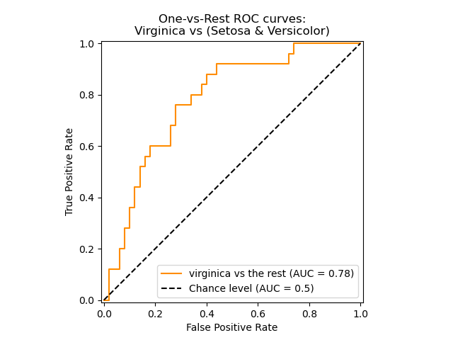
-0.33...3.12 ROC
roc_curve计算了ROC曲线。Wikipedia如下:
“A receiver operating characteristic (ROC), or simply ROC curve, is a graphical plot which illustrates the performance of a binary classifier system as its discrimination threshold is varied. It is created by plotting the fraction of true positives out of the positives (TPR = true positive rate) vs. the fraction of false positives out of the negatives (FPR = false positive rate), at various threshold settings. TPR is also known as sensitivity, and FPR is one minus the specificity or true negative rate.”
该函数需要二分类的真实值和预测值,它可以是正例的概率估计,置信值,或二分决策值。下例展示了如何使用:
>>> import numpy as np
>>> from sklearn.metrics import roc_curve
>>> y = np.array([1, 1, 2, 2])
>>> scores = np.array([0.1, 0.4, 0.35, 0.8])
>>> fpr, tpr, thresholds = roc_curve(y, scores, pos_label=2)
>>> fpr
array([ 0. ,  0.5,  0.5,  1. ])
>>> tpr
array([ 0.5,  0.5,  1. ,  1. ])
>>> thresholds
array([ 0.8 ,  0.4 ,  0.35,  0.1 ])
下图展下了上面的结果:

roc_auc_score函数计算了ROC曲线下面的面积,它也被称为AUC或AUROC。通过计算下面的面积,曲线信息被归一化到1内。
>>> import numpy as np
>>> from sklearn.metrics import roc_auc_score
>>> y_true = np.array([0, 0, 1, 1])
>>> y_scores = np.array([0.1, 0.4, 0.35, 0.8])
>>> roc_auc_score(y_true, y_scores)
0.75
在多标签(multi-label)分类上,roc_auc_score通过对上面的label进行平均。
对比于其它metrics: accuracy、 Hamming loss、 F1-score, ROC不需要为每个label优化一个阀值。roc_auc_score函数也可以用于多分类(multi-class)问题上。如果预测的输出已经被二值化。
示例:
- Receiver Operating Characteristic (ROC)
- Receiver Operating Characteristic (ROC) with cross validation
- Species distribution modeling
3.13 0-1 loss
zero_one_loss会通过在$ n_{\text{samples}} $计算0-1分类的$ L_{0-1}$)的平值或求和。缺省情况下,该函数会对样本进行归一化。为了得到$ L_{0-1} $的求和,需要将normalize设置为False。
在multilabel分类上,如果一个子集的labels与预测值严格匹配,zero_one_loss会得到1,如果有许多错误,则为0。缺省的,该函数会返回有问题的预测子集(不等)的百分比。为了得到这样的子集数,可以将normalize置为False。
如果$ \hat{y}_i $是第i个样本的预测值, $ y_i $是第i个样本的真实值,那么0-1 loss的定义如下:
$ L_{0-1}(y_i, \hat{y}_i) = 1(\hat{y}_i \not= y_i) $
其中1(x)表示的是指示函数。
>>> from sklearn.metrics import zero_one_loss
>>> y_pred = [1, 2, 3, 4]
>>> y_true = [2, 2, 3, 4]
>>> zero_one_loss(y_true, y_pred)
0.25
>>> zero_one_loss(y_true, y_pred, normalize=False)
1
在多标签的问题上,如果使用二元标签指示器,第一个标签集[0,1]具有一个error:
>>> zero_one_loss(np.array([[0, 1], [1, 1]]), np.ones((2, 2)))
0.5

>>> zero_one_loss(np.array([[0, 1], [1, 1]]), np.ones((2, 2)),  normalize=False)
1
示例:
4. Multilabel的ranking metrics
在多标签学习上,每个样本都具有多个真实值label与它对应。它的目的是,为真实值label得到最高分或者最好的rank。
4.1 范围误差(Coverage error)
coverage_error计算了那些必须在最终预测(所有真实的label都会被预测)中包含的labels的平均数目。如果你想知道有多少top高分labels(top-scored-labels)时它会很有用,你必须以平均的方式进行预测,不漏过任何一个真实label。该metrics的最优值是对真实label求平均。
给定一个真实label的二分类指示矩阵:
\[y \in \left\{0, 1\right\}^{n_\text{samples} \times n_\text{labels}}\]以及每个label相关的分值:
\[\hat{f} \in \mathbb{R}^{n_\text{samples} \times n_\text{labels}}\]相应的范围误差定义如下:
\[coverage(y, \hat{f}) = \frac{1}{n_{\text{samples}}} \sum_{i=0}^{n_{\text{samples}} - 1} \max_{j:y_{ij} = 1} \text{rank}_{ij}\]其中:$ \text{rank}{ij} = \left|\left{k: \hat{f}{ik} \geq \hat{f}_{ij} \right}\right| $。给定rank定义,通过给出最大的rank,来打破y_scores。
示例如下:
>>> import numpy as np
>>> from sklearn.metrics import coverage_error
>>> y_true = np.array([[1, 0, 0], [0, 0, 1]])
>>> y_score = np.array([[0.75, 0.5, 1], [1, 0.2, 0.1]])
>>> coverage_error(y_true, y_score)
2.5
4.2 Label ranking平均准确率
label_ranking_average_precision_score函数实现了Label ranking平均准确率 :LRAP(label ranking average precision)。该metric与average_precision_score有关联,但它基于label ranking的概念,而非precision/recall。
LRAP会对每个样本上分配的真实label进行求平均,真实值的比例 vs. 低分值labels的总数。如果你可以为每个样本相关的label给出更好的rank,该指标将产生更好的分值。得到的score通常都会比0大,最佳值为1。如果每个样本都只有一个相关联的label,那么LRAP就与平均倒数排名:mean reciprocal rank
给定一个true label的二元指示矩阵,$ y \in \mathcal{R}^{n_\text{samples} \times n_\text{labels}} $,每个label相对应的分值:$ \hat{f} \in \mathcal{R}^{n_\text{samples} \times n_\text{labels}} $,平均准确率的定义如下:
\[LRAP(y, \hat{f}) = \frac{1}{n_{\text{samples}}} \sum_{i=0}^{n_{\text{samples}} - 1} \frac{1}{|y_i|} \sum_{j:y_{ij} = 1} \frac{|\mathcal{L}_{ij}|}{\text{rank}_{ij}}\]其中:
- $ \mathcal{L}{ij} = \left{k: y{ik} = 1, \hat{f}{ik} \geq \hat{f}{ij} \right} $,
- $ \text{rank}{ij} = \left|\left{k: \hat{f}{ik} \geq \hat{f}_{ij} \right}\right| $
- $ | \cdot | $是l0 范式或是数据集的基数。
该函数的示例:
>>> import numpy as np
>>> from sklearn.metrics import label_ranking_average_precision_score
>>> y_true = np.array([[1, 0, 0], [0, 0, 1]])
>>> y_score = np.array([[0.75, 0.5, 1], [1, 0.2, 0.1]])
>>> label_ranking_average_precision_score(y_true, y_score)
0.416...
4.3 Ranking loss
label_ranking_loss函数用于计算ranking loss,它会对label对没有正确分配的样本进行求平均。例如:true labels的分值比false labels的分值小,或者对true/false label进行了相反的加权。最低的ranking loss为0.
给定一个true labels的二元指示矩阵:$ y \in \left{0, 1\right}^{n_\text{samples} \times n_\text{labels}} $,每个label相关的分值为:$ \hat{f} \in \mathbb{R}^{n_\text{samples} \times n_\text{labels}} $,ranking loss的定义如下:
\[\text{ranking\_loss}(y, \hat{f}) = \frac{1}{n_{\text{samples}}} \sum_{i=0}^{n_{\text{samples}} - 1} \frac{1}{\|y_i\|(n_\text{labels} - |y_i|)} \left\|\left\{(k, l): \hat{f}_{ik} < \hat{f}_{il}, y_{ik} = 1, y_{il} = 0 \right\}\right\|\]其中$ | \cdot | $ 为l0范式或数据集基数。
示例:
>>> import numpy as np
>>> from sklearn.metrics import label_ranking_loss
>>> y_true = np.array([[1, 0, 0], [0, 0, 1]])
>>> y_score = np.array([[0.75, 0.5, 1], [1, 0.2, 0.1]])
>>> label_ranking_loss(y_true, y_score)
0.75...

>>> y_score = np.array([[1.0, 0.1, 0.2], [0.1, 0.2, 0.9]])
>>> label_ranking_loss(y_true, y_score)
0.0
5.回归metrics
sklearn.metrics 实现了许多种loss, score,untility函数来测评回归的性能。其中有一些可以作了增加用于处理多输出(multioutput)的情况:
这些函数具有一个multioutput关键参数,它指定了对于每一个单独的target是否需要对scores/loss进行平均。缺省值为’uniform_average’,它会对结果进行均匀加权平均。如果输出的ndarray的shape为(n_outputs,),那么它们返回的entries为权重以及相应的平均权重。如果multioutput参数为’raw_values’,那么所有的scores/losses都不改变,以raw的方式返回一个shape为(n_outputs,)的数组。
r2_score和explained_variance_score 对于multioutput参数还接受另一个额外的值:’variance_weighted’。该选项将通过相应target变量的variance产生一个为每个单独的score加权的值。该设置将会对全局捕获的未归一化的variance进行量化。如果target的variance具有不同的规模(scale),那么该score将会把更多的重要性分配到那些更高的variance变量上。
对于r2_score的缺省值为multioutput=’variance_weighted’,向后兼容。后续版本会改成uniform_average。
5.1 可释方差值(Explained variance score)
explained_variance_score解释了explained variance regression score
如果$ \hat{y} $是估计的target输出,y为相应的真实(correct)target输出,Var为求方差(variance),即标准差的平方,那么可释方差(explained variance)的估计如下:
\[\texttt{explained\_{}variance}(y, \hat{y}) = 1 - \frac{Var\{ y - \hat{y}\}}{Var\{y\}}\]最好的可能值为1.0,越低表示越差。
示例如下:
>>> from sklearn.metrics import explained_variance_score
>>> y_true = [3, -0.5, 2, 7]
>>> y_pred = [2.5, 0.0, 2, 8]
>>> explained_variance_score(y_true, y_pred)
0.957...
>>> y_true = [[0.5, 1], [-1, 1], [7, -6]]
>>> y_pred = [[0, 2], [-1, 2], [8, -5]]
>>> explained_variance_score(y_true, y_pred, multioutput='raw_values')
...
array([ 0.967...,  1.        ])
>>> explained_variance_score(y_true, y_pred, multioutput=[0.3, 0.7])
...
0.990...
5.2 平均绝对误差(Mean absolute error)
mean_absolute_error函数将会计算平均绝对误差,该指标对应于绝对误差loss(absolute error loss)或l1范式loss(l1-norm loss)的期望值。
如果$ \hat{y}i $是第i个样本的预测值,yi是相应的真实值,那么在$ n{\text{samples}} $上的平均绝对误差(MAE)的定义如下:
\[\text{MAE}(y, \hat{y}) = \frac{1}{n_{\text{samples}}} \sum_{i=0}^{n_{\text{samples}}-1} \left| y_i - \hat{y}_i \right|\]示例:
>>> from sklearn.metrics import mean_absolute_error
>>> y_true = [3, -0.5, 2, 7]
>>> y_pred = [2.5, 0.0, 2, 8]
>>> mean_absolute_error(y_true, y_pred)
0.5
>>> y_true = [[0.5, 1], [-1, 1], [7, -6]]
>>> y_pred = [[0, 2], [-1, 2], [8, -5]]
>>> mean_absolute_error(y_true, y_pred)
0.75
>>> mean_absolute_error(y_true, y_pred, multioutput='raw_values')
array([ 0.5,  1. ])
>>> mean_absolute_error(y_true, y_pred, multioutput=[0.3, 0.7])
...
0.849...
5.3 均方误差(Mean squared error)
mean_squared_error用于计算平均平方误差,该指标对应于平方(二次方)误差loss(squared (quadratic) error loss)的期望值。
\[\text{MSE}(y, \hat{y}) = \frac{1}{n_\text{samples}} \sum_{i=0}^{n_\text{samples} - 1} (y_i - \hat{y}_i)^2.\]示例为:
>>> from sklearn.metrics import mean_squared_error
>>> y_true = [3, -0.5, 2, 7]
>>> y_pred = [2.5, 0.0, 2, 8]
>>> mean_squared_error(y_true, y_pred)
0.375
>>> y_true = [[0.5, 1], [-1, 1], [7, -6]]
>>> y_pred = [[0, 2], [-1, 2], [8, -5]]
>>> mean_squared_error(y_true, y_pred)
0.7083...
示例:
5.4 中值绝对误差(Median absolute error)
median_absolute_error是很令人感兴趣的,它对异类(outliers)的情况是健壮的。该loss函数通过计算target和prediction间的绝对值,然后取中值得到。
MedAE的定义如下:
\[\text{MedAE}(y, \hat{y}) = \text{median}(\mid y_1 - \hat{y}_1 \mid, \ldots, \mid y_n - \hat{y}_n \mid)\]median_absolute_error不支持multioutput。
示例:
>>> from sklearn.metrics import median_absolute_error
>>> y_true = [3, -0.5, 2, 7]
>>> y_pred = [2.5, 0.0, 2, 8]
>>> median_absolute_error(y_true, y_pred)
0.5
5.5 R方值,确定系数
r2_score函数用于计算R²(确定系数:coefficient of determination)。它用来度量未来的样本是否可能通过模型被很好地预测。分值为1表示最好,它可以是负数(因为模型可以很糟糕)。一个恒定的模型总是能预测y的期望值,忽略掉输入的feature,得到一个R^2为0的分值。
R²的定义如下:
\[R^2(y, \hat{y}) = 1 - \frac{\sum_{i=0}^{n_{\text{samples}} - 1} (y_i - \hat{y}_i)^2}{\sum_{i=0}^{n_\text{samples} - 1} (y_i - \bar{y})^2}\]其中:$ \bar{y} = \frac{1}{n_{\text{samples}}} \sum_{i=0}^{n_{\text{samples}} - 1} y_i $
示例:
>>> from sklearn.metrics import r2_score
>>> y_true = [3, -0.5, 2, 7]
>>> y_pred = [2.5, 0.0, 2, 8]
>>> r2_score(y_true, y_pred)
0.948...
>>> y_true = [[0.5, 1], [-1, 1], [7, -6]]
>>> y_pred = [[0, 2], [-1, 2], [8, -5]]
>>> r2_score(y_true, y_pred, multioutput='variance_weighted')
...
0.938...
>>> y_true = [[0.5, 1], [-1, 1], [7, -6]]
>>> y_pred = [[0, 2], [-1, 2], [8, -5]]
>>> r2_score(y_true, y_pred, multioutput='uniform_average')
...
0.936...
>>> r2_score(y_true, y_pred, multioutput='raw_values')
...
array([ 0.965...,  0.908...])
>>> r2_score(y_true, y_pred, multioutput=[0.3, 0.7])
...
0.925...
示例:
6.聚类metrics
sklearn.metrics也提供了聚类的metrics。更多细节详见:
7. Dummy estimators
当进行监督学习时,一个简单明智的check包括:使用不同的规则比较一个estimator。DummyClassifier实现了三种简单的策略用于分类:
- stratified:根据训练集的分布来生成随机预测
- most_frequent:在训练集中总是预测最频繁的label
- prior:总是预测分类最大化分类优先权(比如:most_frequent),predict_proba返回分类优化权
- uniform:以均匀方式随机生成预测
- constant:由用户指定,总是预测一个常量的label。该方法的一个最主要动机是:F1-scoring,其中正例是最主要的。
注意,所有的这些策略中,predict方法会完成忽略输入数据!
示例,我们首先创建一个imbalanced的数据集:
>>> from sklearn.datasets import load_iris
>>> from sklearn.cross_validation import train_test_split
>>> iris = load_iris()
>>> X, y = iris.data, iris.target
>>> y[y != 1] = -1
>>> X_train, X_test, y_train, y_test = train_test_split(X, y, random_state=0)
下一步,比较下SVC的accuary和most_frequent:
>>> from sklearn.dummy import DummyClassifier
>>> from sklearn.svm import SVC
>>> clf = SVC(kernel='linear', C=1).fit(X_train, y_train)
>>> clf.score(X_test, y_test)
0.63...
>>> clf = DummyClassifier(strategy='most_frequent',random_state=0)
>>> clf.fit(X_train, y_train)
DummyClassifier(constant=None, random_state=0, strategy='most_frequent')
>>> clf.score(X_test, y_test)
0.57...
我们可以看到SVC并不比DummyClassifier好很多,接着,我们换下kernel:
>>> clf = SVC(kernel='rbf', C=1).fit(X_train, y_train)
>>> clf.score(X_test, y_test)
0.97...
我们可以看到,accuracy增强到了几乎100%。如果CPU开销不大,这里建议再做下cross-validation。如果你希望在参数空间进行优化,我们强烈推荐你使用GridSearchCV。
更一般的,分类器的accuracy太接近于随机,这可能意味着有可能会出问题:features没有用,超参数没有被正确设置,分类器所用的数据集imbalance,等等。。。
DummyRegressor也实现了4种简单的方法:
- mean:通常预测训练target的均值。
- median:通常预测训练target的中值。
- quantile:预测由用户提供的训练target的分位数
- constant:常量
在上面的所有策略,predict完全忽略输入数据。
参考:
http://scikit-learn.org/stable/modules/model_evaluation.html